Titanic EDA
September 27, 2022 — 539 readThe sinking of the Titanic is one of the most notorious shipwrecks in history. On April 15, 1912, during her maiden voyage, the widely considered “unsinkable” RMS Titanic sank after colliding with an iceberg. Unfortunately, there were not enough lifeboats for everyone onboard, resulting in the death of 1502 out of 2224 passengers and crew.
While there was some element of luck involved in surviving, it seems some groups of people were more likely to survive than others.
check this link to see my original codes on kaggle.com.
import numpy as np # linear algebra
import pandas as pd # data processing, CSV file I/O (e.g. pd.read_csv)

import matplotlib.pyplot as plt
plt.style.use("seaborn-pastel")

import seaborn as sns

from collections import Counter

import warnings
warnings.filterwarnings("ignore")
1. LOAD AND CHECK DATA
train_df = pd.read_csv("/kaggle/input/titanic/train.csv")
test_df = pd.read_csv("/kaggle/input/titanic/test.csv")
test_PassengerID = test_df["PassengerId"]train_df.columnsout: Index(['PassengerId', 'Survived', 'Pclass', 'Name', 'Sex', 'Age', 'SibSp', 'Parch', 'Ticket', 'Fare', 'Cabin', 'Embarked'], dtype='object')
train_df.head()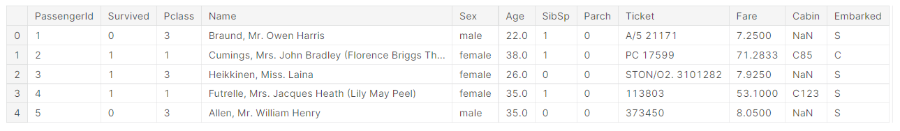
train_df.describe()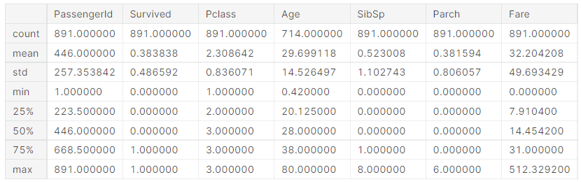
2. VARIABLE DESCRIPTION
PassengerId: unique id number for each passenger
Survived: there are 0 and 1, if variable is 0 so passenger was death, else 1 so survived.
Pclass: passenger class
Name: name
Sex: gender of passenger
Age: age of passenger
SibSp: number of siblings/spouses
Parch: number of parents/children
Ticket: number of ticket
Fare: price of ticket
Cabin: the category of cabinet
Embarke: ports where passenger embarked (C: Cherbourg, Q:Queenstown, S=Southampton)
train_df.info()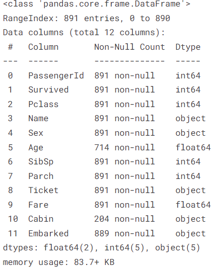
2.1. Univariate Variable Analysis
- Categorical Variable: Survived, Sex, Pclass, Embarked, Cabin, Name, Ticket, SibSp and Parch
- Numerical Variable: Age, PassengerId, Fare
2.1.1. Categorical Variable
def bar_plot(variable):
    """
        input: variable ex:"Sex"
        output: bar plot & value count
    """
    #get features
    var = train_df[variable]
    #count number of categorical variable(value/sample)
    varValue = var.value_counts()

    #visualize
    plt.figure(figsize = (9,3))
    plt.bar(varValue.index, varValue)
    plt.xticks(varValue.index, varValue.index.values)
    plt.ylabel("Frequency")
    plt.title(variable)
    plt.show()
    print("{}: \n {}".format(variable, varValue))
category1 = ["Survived", "Sex", "Pclass", "Embarked", "SibSp", "Parch"]
for c in category1:
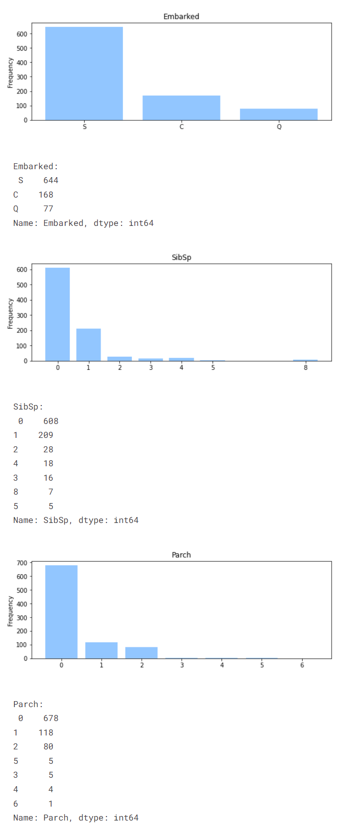
bar_plot(c)
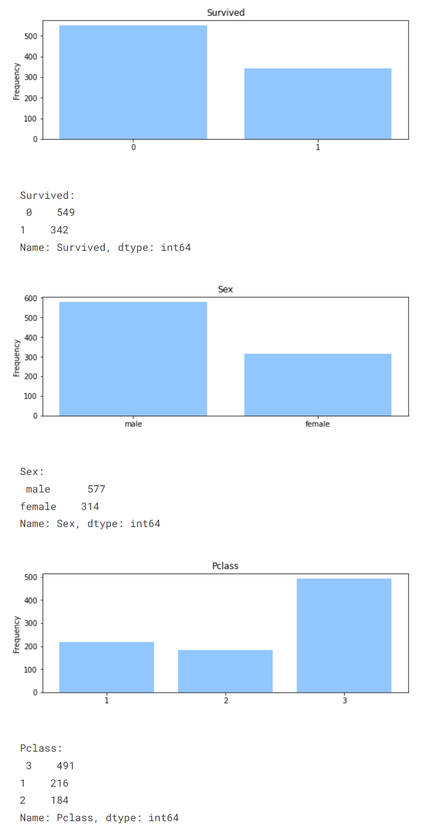
In Survived histogram, it is obvious that 549 passenger did not survive, at the same time 342 people survived. Of the 551 passengers, 549 did not survive and 342 survived. Of the 551 passengers, 549 did not survive and 342 survived. These are not half, so the survive dataset is not a balanced dataset.
Of the 891 passengers, 577 were men and 314 were women. This data set has an uneven distribution. By looking at this data set, one can have the idea that a passenger is an average of 1/3 male by looking at the male to female ratio.
There are three classes in Pclass data. There are 216 passengers in the first class, 184 in the second class and 491 in the third class.
The relationship between Embarked and Pclass will be examined.
category2 = ["Cabin", "Name", "Ticket"]
for c in category2:
    print("{} \n".format(train_df[c].value_counts()))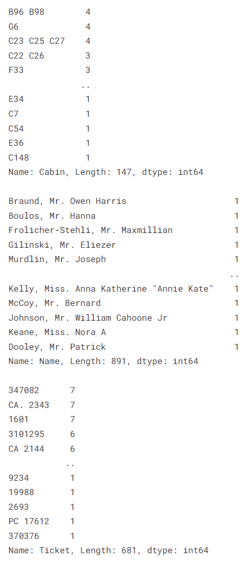
2.1.2. Numerical Variable
def plot_histogram(variable):
    plt.figure(figsize= (9,3))
    plt.hist(train_df[variable], bins=50)
    plt.xlabel(variable)
    plt.ylabel("Frequency")
    plt.title("{} distribution with hist".format(variable))
    plt.show()
numericVar=["Fare", "Age", "PassengerId"]
for n in numericVar:
plot_histogram(n)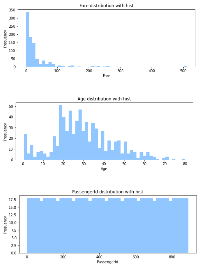
In Fare distribution with his, the price can be seen above 100 that is mostly paid. There is an option for who paid 500 means he/she wa rich or paid someone else ticket.
In age distribution, the consistency is stayed ages that are in between 20 and 30. Also, the number of kids are also quite high.
3. BASIC DATA ANALYSIS
# pclass vs survived

train_df[["Pclass", "Survived"]].groupby(["Pclass"], as_index = False).mean().sort_values(by="Survived", ascending = False)| Pclass | Survived | |
|---|---|---|
| 0 | 1 | 0.629630 |
| 1 | 2 | 0.472826 |
| 2 | 3 | 0.242363 |
Passengers who bought first class tickets were more likely to survive than other class. That is %62. The second class percent is %47, the third class is %24.
# Sex vs survived

train_df[["Sex", "Survived"]].groupby(["Sex"], as_index = False).mean().sort_values(by="Survived", ascending = False)| Sex | Survived | |
|---|---|---|
| 0 | female | 0.742038 |
| 1 | male | 0.188908 |
# SibSp vs survived

train_df[["SibSp", "Survived"]].groupby(["SibSp"], as_index = False).mean().sort_values(by="Survived", ascending = False)| SibSp | Survived | |
|---|---|---|
| 1 | 1 | 0.535885 |
| 2 | 2 | 0.464286 |
| 0 | 0 | 0.345395 |
| 3 | 3 | 0.250000 |
| 4 | 4 | 0.166667 |
| 5 | 5 | 0.000000 |
| 6 | 8 | 0.000000 |
Survival rate of those with a sibling with them is the highest with 53.6%. The odds of survival for those with no one are in the third place with 34%. Survival rate is very low for those who have more than two people with them.
# Parch vs survived

train_df[["Parch", "Survived"]].groupby(["Parch"], as_index = False).mean().sort_values(by="Survived", ascending = False)| Parch | Survived | |
|---|---|---|
| 3 | 3 | 0.600000 |
| 1 | 1 | 0.550847 |
| 2 | 2 | 0.500000 |
| 0 | 0 | 0.343658 |
| 5 | 5 | 0.200000 |
| 4 | 4 | 0.000000 |
| 6 | 6 | 0.000000 |
If there is a family or a child with them, that is, 3 people in total, the probability of survival is around 50%. However, as this number increases, the survival rate decreases.
4. OUTLINER DETECTION
def detect_outliers(df,features):
    outliner_indexes = []

    for c in features:
        #1st quartile
        Q1 = np.percentile(df[c], 25)

        #3rd quartile
        Q3 = np.percentile(df[c], 75)

        #IQR
        IQR = Q1 - Q3

        #Outliner ster
        outliner_step = IQR * 1.5

        #Detect outliner and their indexes
        outliner_list_col = df[(df[c] < Q1 - outliner_step) | (df[c] > Q3 + outliner_step)].index

        #store indexes
        outliner_indexes.extend(outliner_list_col)

    outliner_indexes = Counter(outliner_indexes)
    multiple_outliers = list(i for i, v in outliner_indexes.items() if v > 2)

    return multiple_outliers
train_df.loc[detect_outliers(train_df, ["Age", "SibSp", "Parch", "Fare"])]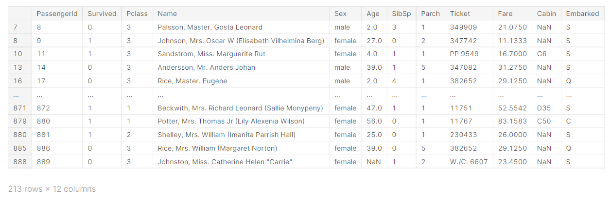
#drop outliners
train_df = train_df.drop(detect_outliers(train_df, ["Age", "SibSp", "Parch", "Fare"]), axis=0).reset_index ( drop = True)
4. MISSING VALUE
train_df_len = len(train_df)
train_df = pd.concat([train_df, test_df], axis = 0).reset_index(drop = True)
train_df.head()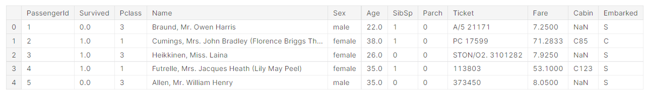
4.1. Find Missing Value
#finding which columns contain null
train_df.columns[train_df.isnull().any()]
Index(['Survived', 'Age', 'Fare', 'Cabin', 'Embarked'], dtype='object')
#how many nulls that those columns have
train_df.isnull().sum()
PassengerId 0
Survived 418
Pclass 0
Name 0
Sex 0
Age 243
SibSp 0
Parch 0
Ticket 0
Fare 1
Cabin 864
Embarked 2
dtype: int64
4.2. Fill Missing Value
train_df[train_df["Embarked"].isnull()]
| PassengerId | Survived | Pclass | Name | Sex | Age | SibSp | Parch | Ticket | Fare | Cabin | Embarked | |
|---|---|---|---|---|---|---|---|---|---|---|---|---|
| 48 | 62 | 1.0 | 1 | Icard, Miss. Amelie | female | 38.0 | 0 | 0 | 113572 | 80.0 | B28 | NaN |
| 633 | 830 | 1.0 | 1 | Stone, Mrs. George Nelson (Martha Evelyn) | female | 62.0 | 0 | 0 | 113572 | 80.0 | B28 | NaN |
Embarked can be charged by comparison for filling. For example, you can see where the first class passengers are getting on, or fare and fill them accordingly.
train_df.boxplot(column="Fare", by="Embarked")
plt.show
<function matplotlib.pyplot.show(close=None, block=None)>
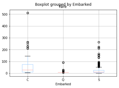
The median of those who embark from port C is closer to eighty than the others, because the fare for empty ones is 80. hence the blank data will be filled as C.
train_df["Embarked"] = train_df["Embarked"].fillna("C")
train_df[train_df["Embarked"].isnull()]train_df[train_df["Fare"].isnull()]train_df["Fare"] = train_df["Fare"].fillna(np.mean(train_df[train_df["Pclass"] == 3]["Fare"]))train_df[train_df["Fare"].isnull()]